Landing a UAV in Harsh Winds and Turbulent Open Waters

Introduction to the problem

Aerial autonomy and Marine autonomy have reached a great level of maturity on their own currently and various complex tasks can be carried out by these agents on their own in their own “respective” environment but we wanted to work on autonomous teams that can combine the advantages of these systems.

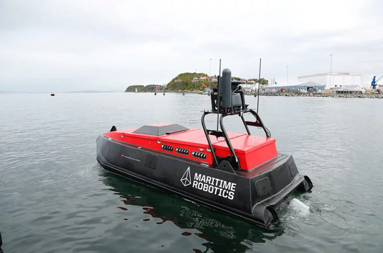
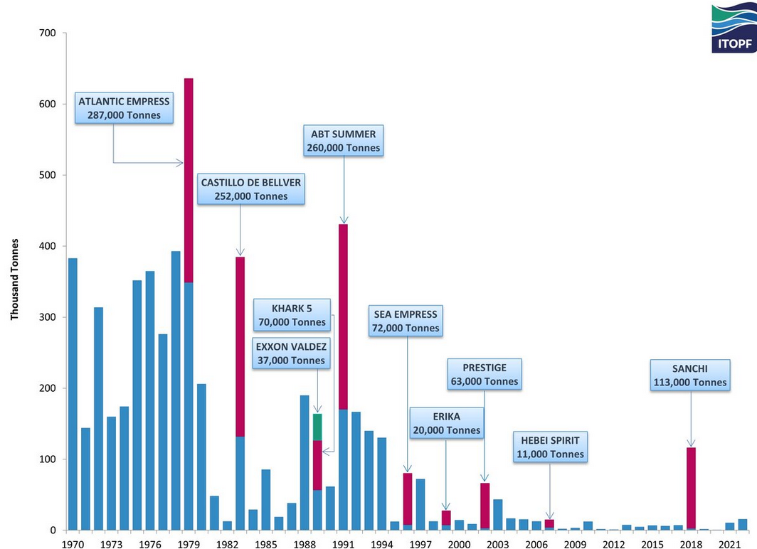
The primary application for this approach was going to be cleaning of trash and oil-spills from the ocean. While the problem of oil spills has been improving due to new safety measures, there are still 1000s of tons of oil spillage every year. On the other hand, garbage/trash discharge into the ocean has been an increasingly severe issue for the planet and USVs can help humans save time, effort, and energy in making a dent in the clean-up efforts. Moreover, there are safety benefits to not putting humans in dangerous environment to begin with.

We wanted to take advantage of the marine vehicle for lugging around cleaning equipment or tugging on the nets carrying trash, and also provide the awareness and mission control/direction capabilities that aerial vehicles can offer.

But, for true autonomy that saves human-hours spent on the mission, the aerial vehicles need to be able to land and charge autonomously. Therefore, this was the problem we picked to solve. For landing, we decided to take a look at the risks posed to the UAV during the landing. As it turned out, there were several different ship motions that need to be accounted for in order to prevent collisions and the subsequent damages. Here are all the motions of a ship that can be problematic to the UAV during landing:

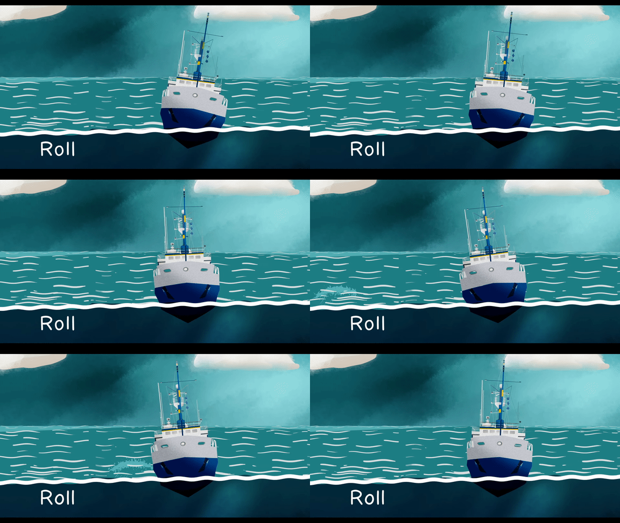
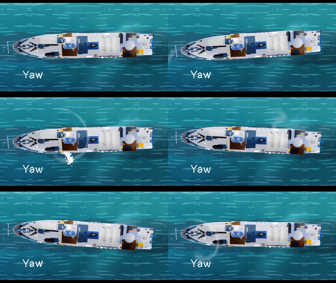
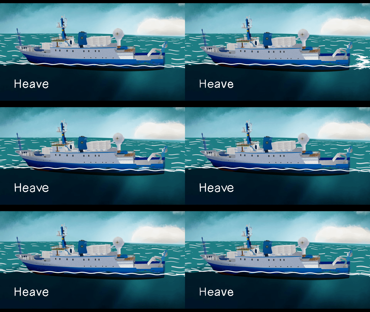
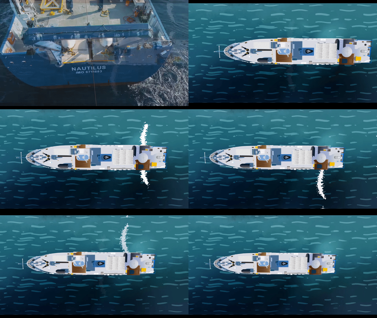
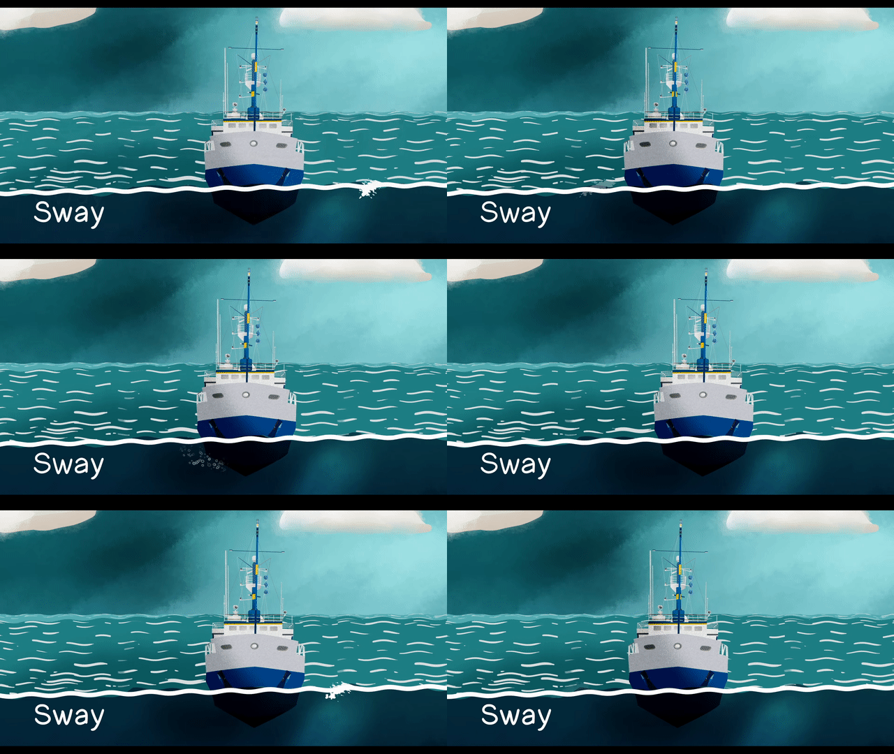
Out of these combined 6 motions in 3 axes, as it turns out, only three of them are dangerous to a landing. While yaw, surge, and sway motions can be counteracted by building a sufficiently-large landing deck, roll, pitch, and heave motion cannot be compensated by design measures excluding self-levelling actuated platforms. Therefore, we need to focus on the latter three and how control and prediction can solve the problems in these axes. Looking at literature, the dangers posed to the landing mission can be identified using simple illustrations below.

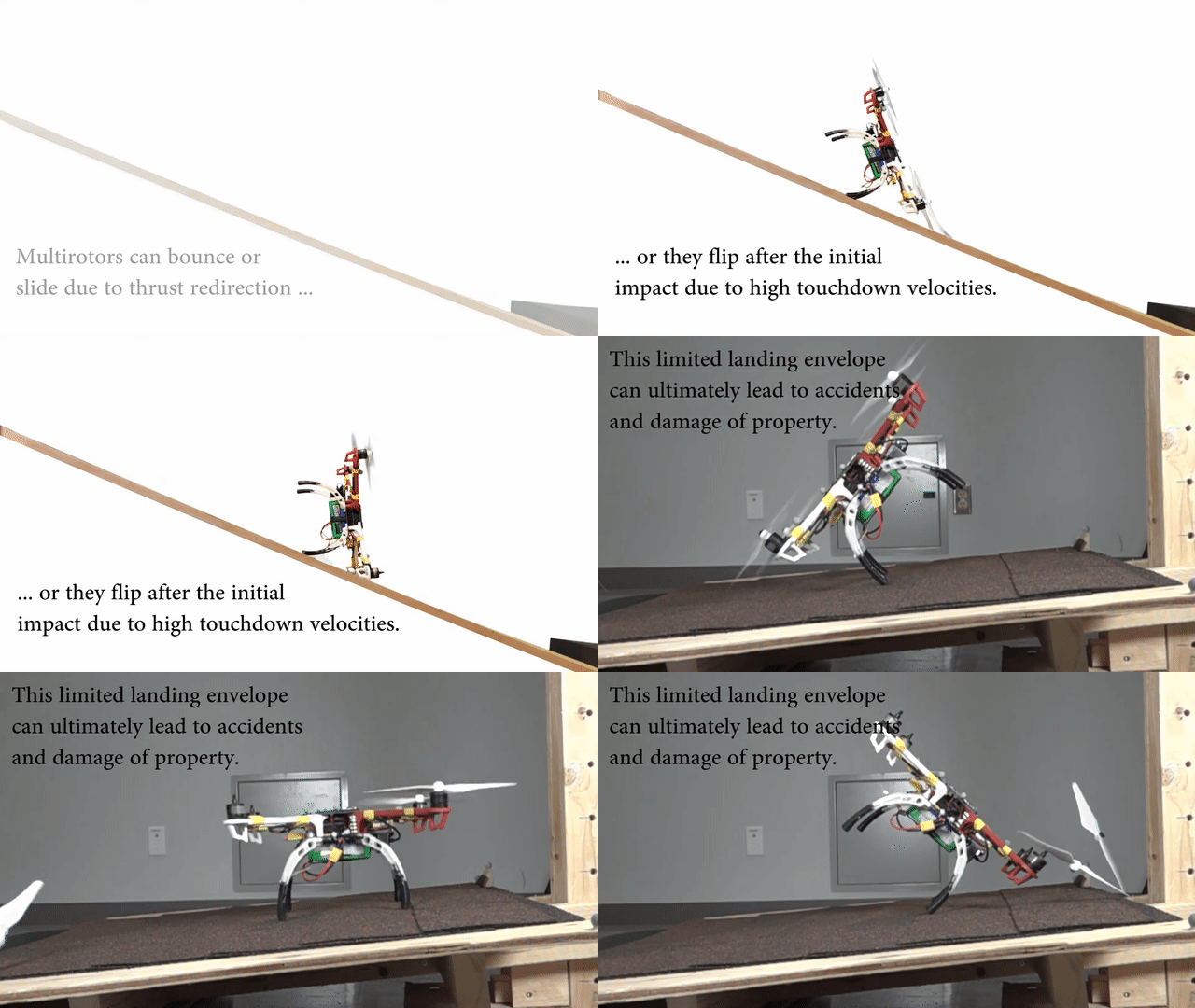
As is clear from these images, a tilted deck can lead to an impulse transfer to the UAV that can lead to undesired pitching, rolling, and rebounding from the landing deck in the landing phase. Whereas, a heaving platform can induce a fracture-causing stress in the landing gear due to high relative velocity during touchdown. In order to manage these undesired moments, we wanted to study the motion and understand if we could find an opportune moment to land during the low-tilt and low-heave of the platform. Another countermeasure for heave can be an advance warning where the UAV can change its vertical approach velocity to match the landing deck dynamically as that degree of control is retained independently and can be adjusted during the landing. In order to do so, we looked to the literature to figure out what could be predicted about this motion.

Literature Review

In this blog, we would like to highlight three significant literatures on the subject and the roles they play in informing our direction for the project.

Riola et. al. discuss how the sea states affect the motion of a ship and how it varies as a function of time. They ascertain through observations that periodic predictable motion of the ship exists for a rolling window of about 30 seconds as new frequencies participate in the motion. As such, in a window of 30 seconds, key frequencies can be identified that can be used to make predictions about the behaviour of the ship. They also discuss the matter of quiescent periods which are defined mathematically to be periods where the system has the lowest energy state and is a safe period to land.

Küchler et. al. discuss and formulate a method of controlling the offshore crane responsible for offloading cargo from marine vessels. In these situations, the tether can go through severe stress if there is a sudden transition from slack to taught state. In order to avoid this, an active control scheme is discussed which can counteract the motion by spooling the tether in and out to match the motion of the cargo container. They do this using a Fast Fourier Transform (FFT) and predicting the movement using a Linear Kalman Filter.

Greer et. al. present their work on landing a helicopter in severe sea states using the non-linear dynamics of the helicopter. In order to do this, they choose a Model Predictive Controller(MPC) to solve a non-linear cost function that allows them to land the helicopter. This approach uses a shrinking horizon method that ends at the landing time. For this, they use pre-specified trajectories, perfect knowledge of the ship motion, and offline computation to demonstrate the solution in numerical simulation environment.

Our approach

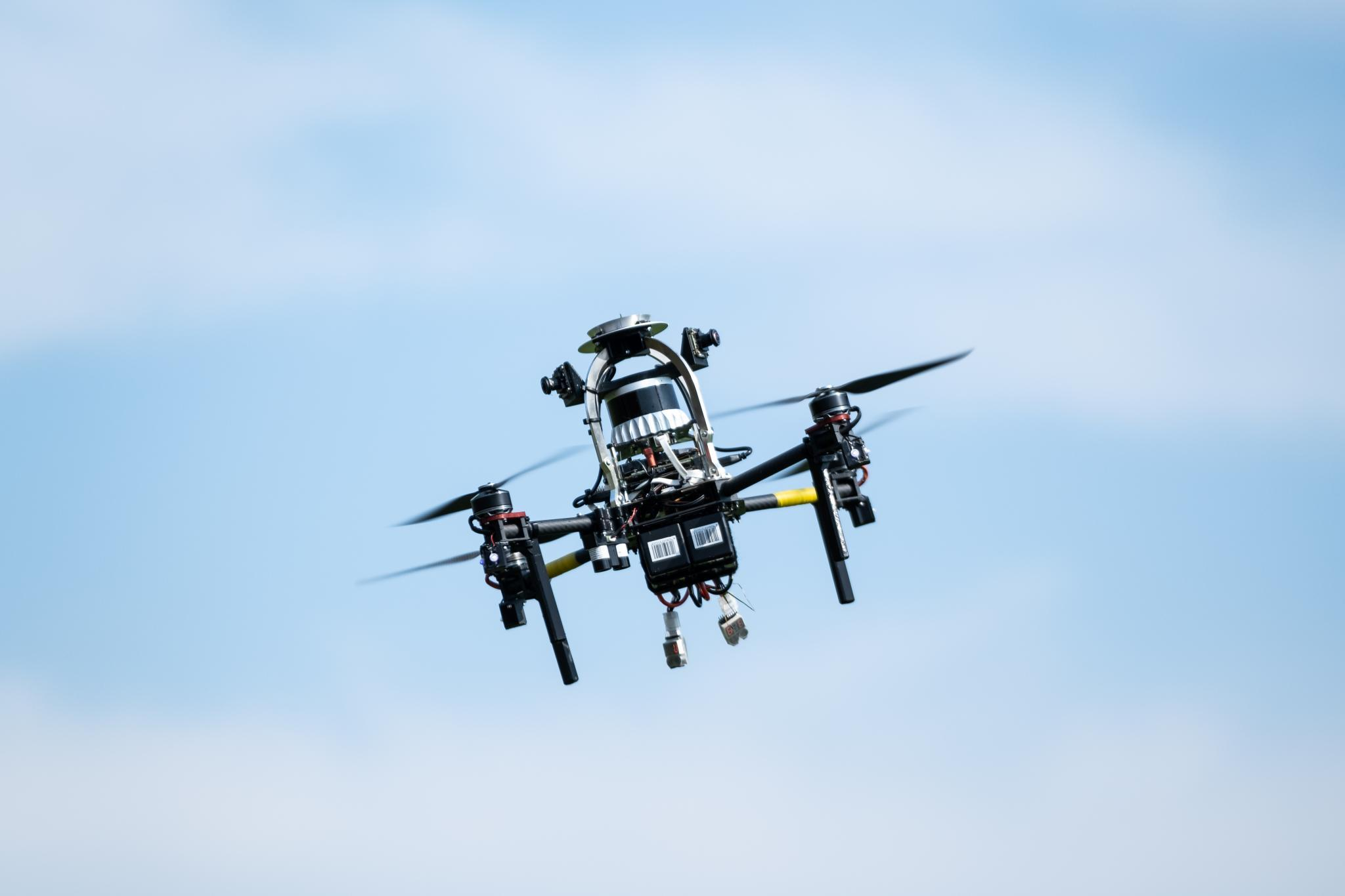
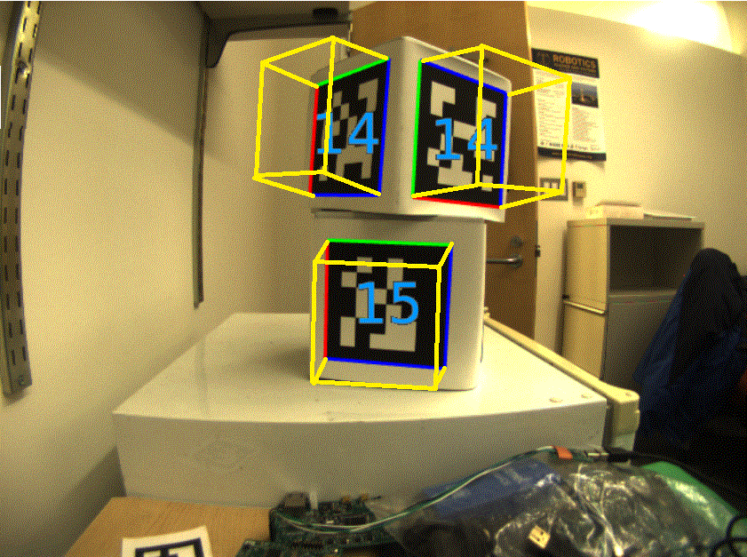
We set out a clear goal for ourselves to demonstrate this approach in the real-world in real conditions and deploy algorithms that can be solved on the UAV in real-time using the limited computation available. For our approach, we first identify the sensory and communication constraints we want to impose on the system. For the purpose of landing, we needed to obtain the pose estimates of the USV and we had to decide whether this pose estimate can be obtained without communication with the USV for obtaining its onboard telemety of its state. In order to decentralise the system and make it robust as well as applicable to wide-range of scenarios, we choose to use a non-communication approach to our landing mission in the marine environment. Communication with the marine vessel can be unreliable and therefore an independent sensor array onboard the UAV is preferred. For this, we studied the applicability of LiDAR as well as visual pose estimation in this scenario. We found out that LiDAR-based pose estimation can be challenging due to reflections and other changing circumstances when operating under direct sunlight. Moreover, it is a challenge of its own to adapt to various models or constructions of the ship upon which the landing is to be performed. Therefore, we choose visual pose estimation using fiducial markers placed on the landing deck of the ship.

Therefore we formualated our key challenges as follows:

• Estimate and predict the motion of the USV without communication.
• Design a cost function to find and track and optimum landing trajectory using USV predictions.
• Predict the motion of the UAV to minimize relative velocity on touchdown.

Challenge 1: Estimation and Prediction.

We employ a FFT algorithm to identify the motions of the ship using the pose estimates obtained from the onboard camera of the UAV. While FFT can provide a reliable estimate of the frequency of oscillation, the amplitude and phase of the modes need to be augmented and estimated using a Linear Kalman Filter (LKF) to get accurate results. To do this, we formulate a state variable as shown below which represents the motion in a Linear Time Variant state space model. This model can then be used by the LKF in conjunction with the pose measurements to refine the observations and converge to true phase and amplitude for each mode of oscillation.

Using this observer, we can predict the future of the USV motion and use these predictions to inform the MPC of the UAV for picking correct time for landing.

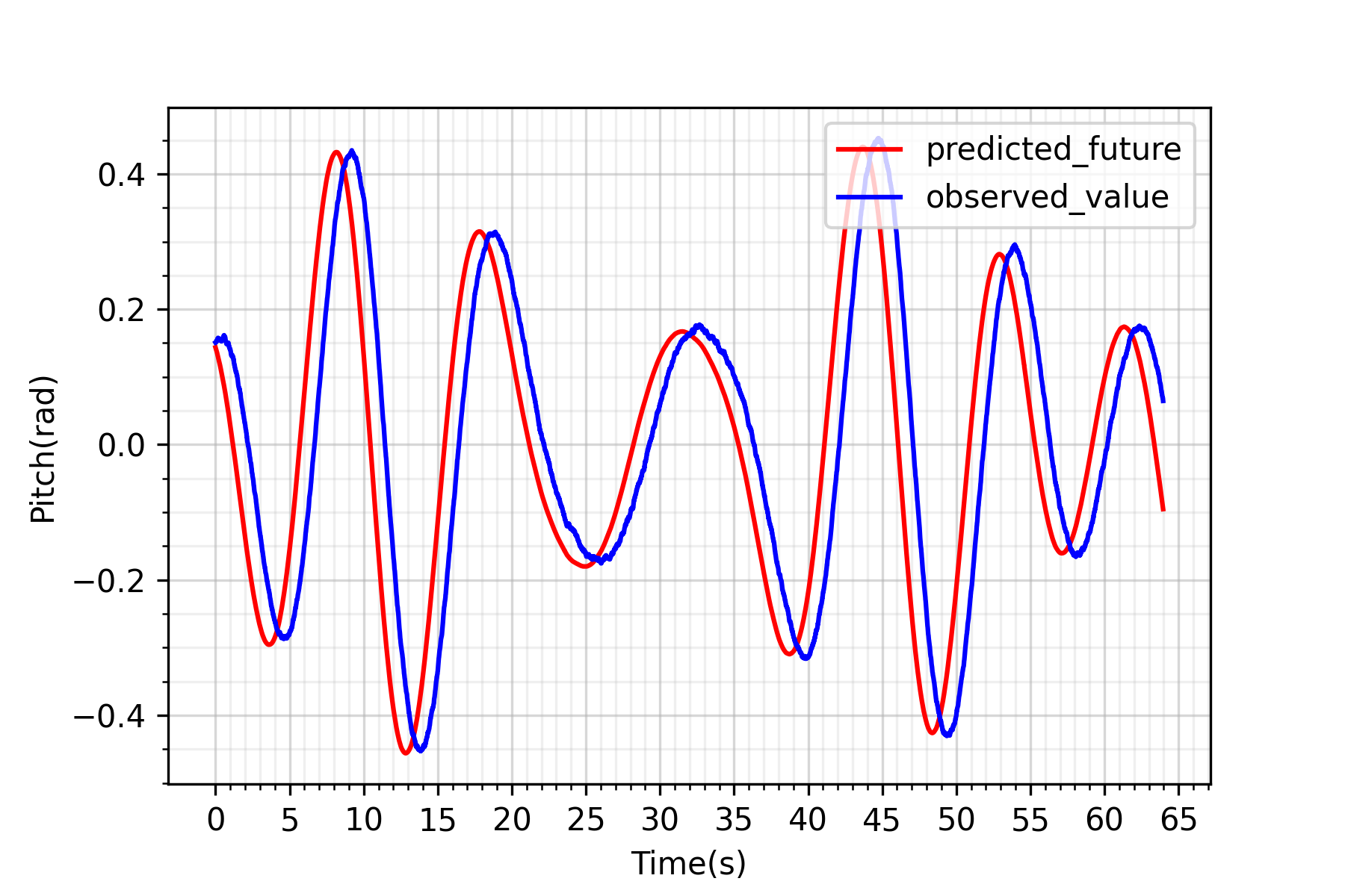
As seen from the predictions made in simuation environment, this approach works better at higher data rate but sufficiently converges at 30 FPS camera-based pose predictions from the Apriltag marker.

Challenge 2 & 3 : Optimum landing and Control

We then focus our attention on the UAV control and the following state as well as model can be obtained by assuming the UAV to be a point-mass with a heading as shown below:

This simplification is necessary to reduce solution complexity but it proves to be sufficient to accomplish this task of landing safely. The output is the required velocity commands and in order to control and drive the velocity and therefore, the attitude as well as the attitude rate, we use our MRS system to fly the UAV using its lower level control nodes that directly communicates with the onboard flight controller.

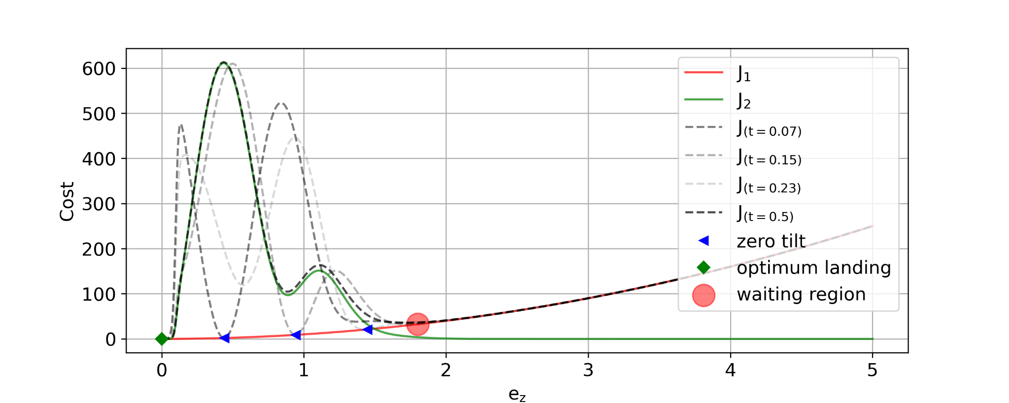
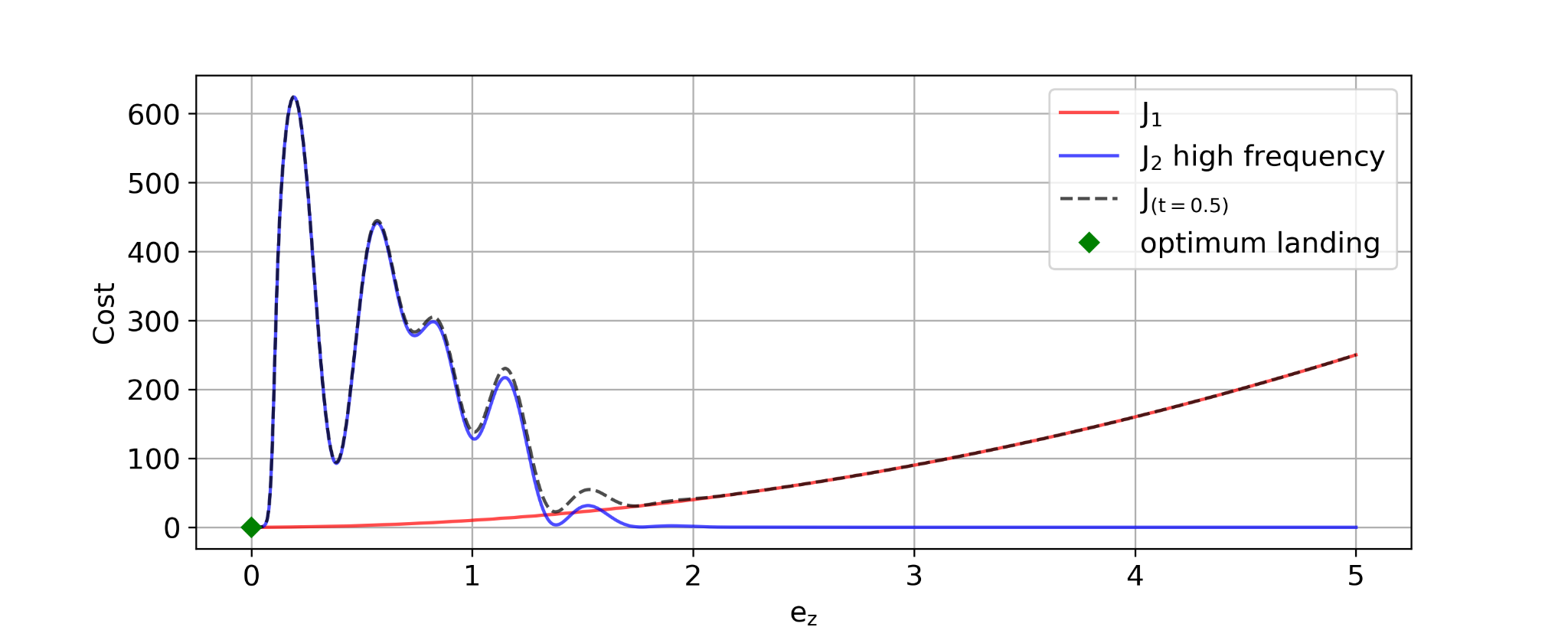
For our MPC, we formulate a novel cost-function which can guide the UAV during waypoint navigation as well as landing approach using the constrained optimization of the cost without employing a finite-state automaton. This approach has the advantage that it can make decisions about landing and waiting to land based on the severity of the USV motion instead of pre-set activation thresholds. To achieve this, we have two sections in our cost function viz J1 and J2 as shown below. While J1 guides the UAV to the waypoint, J2 deal with adapting the cost to the landing criterion.

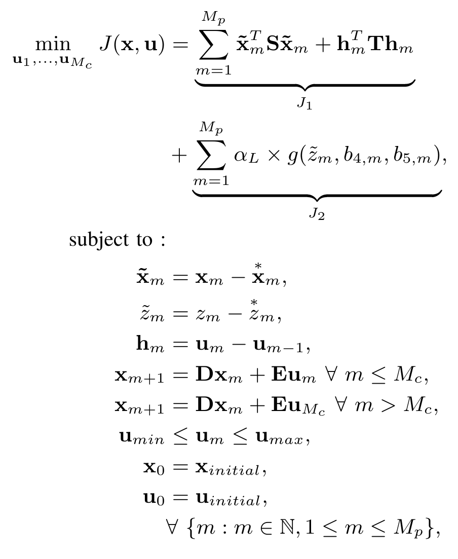
J2 is comprised of a quadratic function and a set of sigmoids to mold the cost function into a set of valleys and troughs that act as natural barrier for the UAV in solving the optimization problem. A simplified plot of the cost function is shown below:

Results

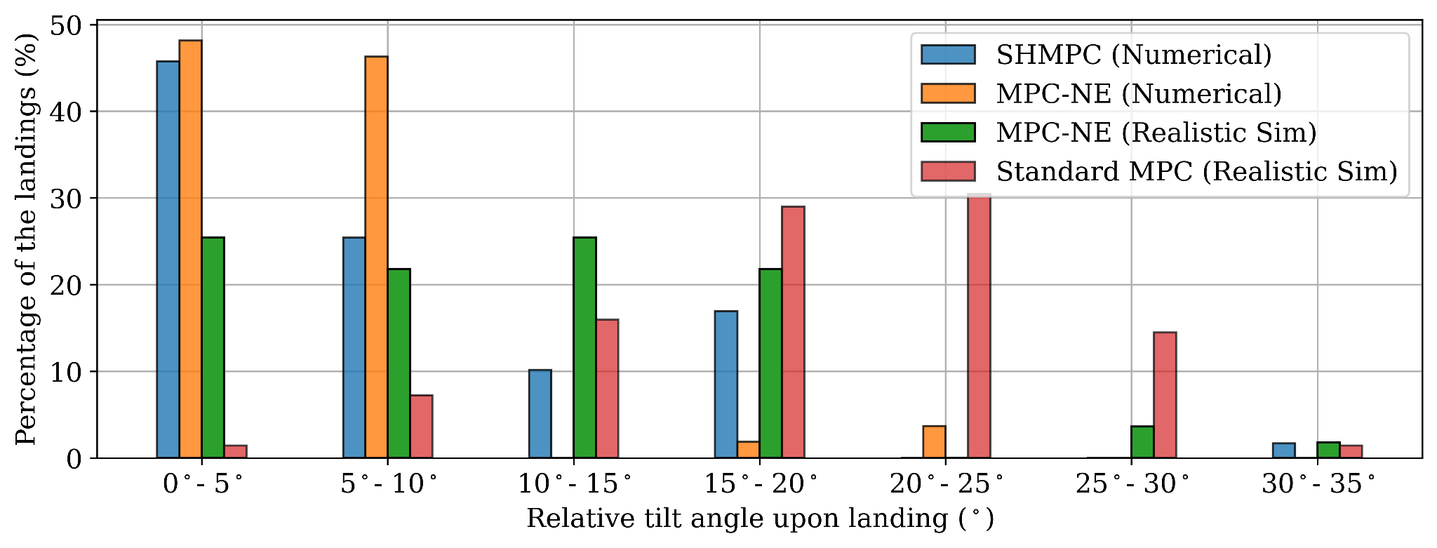
Our results for the simulation as well as real-world environment are presented below with comparisons from other approaches. In simulation environment, we showcase our results in comparison with the approach from Greer et. al. Given equal amount of time to solve, our solution is able to beat the accuracy achieved and also perform the same task without much loss of accuracy when used in real-time environment. In real-world, we also present our results to showcase the predictions made from the pose estimate of the USV.

Drawbacks

• USV is assumed to be stationary or slowly drifting but not actively moving which is important to follow and land.
• MPC could only look 1 second into the future, therefore the UAV has to hover close to the USV to take the opportunity to land.
• The USV has to be manually located and visual search can be limiting.

Future Work (Sneak Peek)

Stay Tuned!